Prophet and R: Forecasting Air Passenger Numbers
Published Oct 5, 2020 by Michael Grogan
In this example, a Prophet model is built using R to forecast air passenger numbers. The data in question is sourced from San Francisco Open Data.
Background
The dataset is sourced from the San Francisco International Airport Report on Monthly Passenger Traffic Statistics by Airline, which is available from data.world (Original Source: San Francisco Open Data) as indicated in the References section below.
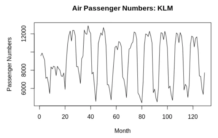
Specifically, adjusted passenger numbers for the airline KLM (enplaned) are filtered as the time series for analysis from the period May 2005 to March 2016.
The purpose of using Prophet is to:
- Identify seasonal patterns in the data
- Model “change points” — or periods of significant structural change in the data
- Forecast future air passenger numbers using seasonal and change point parameters
In this regard, Prophet can potentially produce superior results to more traditional time series models such as ARIMA by identifying structural breaks in a time series and making forecasts by taking change points as well as seasonality patterns into account.
Model Building
In order to allow Prophet to analyse the data in question, one must ensure that it is in the proper format, i.e. a column titled ds for date, and y for the time series values.
The prophet library is loaded, and the relevant data is imported.
library(prophet)
mydata<-read.csv("klm.csv")
ds<-mydata$Date[1:115]
y<-mydata$Adjusted.Passenger.Count[1:115]
train<-data.frame(ds,y)
train
The Prophet model that is defined in this case will detect seasonal patterns automatically. However, we would like to indicate the relevant change points in the model as well.
Four change points are specified as follows:
m <- prophet(train, n.changepoints = 4)
m
The identified change points are then illustrated:
$changepoints
[1] "2007-06-01 GMT" "2009-04-01 GMT" "2011-03-01 GMT"
[4] "2013-02-01 GMT"
The model is then used to predict 14 months forward, with the predictions compared to the test set (actual values).
future <- make_future_dataframe(m, periods = 14, freq = 'month')
tail(future)
forecast <- predict(m, future)
tail(forecast[c('ds', 'yhat', 'yhat_lower', 'yhat_upper')])
plot(m, forecast) + add_changepoints_to_plot(m)
Here is a plot of the change point intervals:

Here is a plot of the trend and yearly components:
prophet_plot_components(m, forecast)
We can see that passenger numbers are higher in the spring and summer overall, with lower passenger numbers throughout the winter months.
Additionally, we see that while air passenger numbers saw a strong increase in trend up until 2010, numbers started to see a slow but steady decline after that point.
Using the Metrics library, the root mean squared error can be calculated and then compared to the mean monthly value:
> ds<-mydata$Date[116:129]
> y<-mydata$Adjusted.Passenger.Count[116:129]
>
> test<-data.frame(ds,y)
> test
           ds     y
1  2015-02-01  5012
2  2015-03-01  6327
3  2015-04-01 10831
4  2015-05-01 11745
5  2015-06-01 11633
6  2015-07-01 10562
7  2015-08-01 11510
8  2015-09-01 11669
9  2015-10-01 10221
10 2015-11-01  7366
11 2015-12-01  7321
12 2016-01-01  5930
13 2016-02-01  5338
14 2016-03-01  7726
>
> library(Metrics)
> rmse(forecast$yhat[116:129],test$y)
[1] 587.1803
>
> mean(test$y)
[1] 8799.357
The RMSE of 587 is relatively low compared to the monthly mean of 8,799. This indicates that our Prophet model does quite a good job at forecasting air passenger numbers.
However, it is notable that the change points that were selected in R are slightly different to that of Python. Specifically, R identified one of the change points as April 2009, but Python identified the change point as May 2009 instead.
What if we manually define the change points in R with May 2009 instead? Will this improve the accuracy of the forecasting model?
m <- prophet(train, changepoints=c("2007-06-01", "2009-05-01", "2011-03-01", "2013-02-01"))Here are the forecasting results:
> ds<-mydata$Date[116:129]
> y<-mydata$Adjusted.Passenger.Count[116:129]
>
> test<-data.frame(ds,y)
> test
           ds     y
1  2015-02-01  5012
2  2015-03-01  6327
3  2015-04-01 10831
4  2015-05-01 11745
5  2015-06-01 11633
6  2015-07-01 10562
7  2015-08-01 11510
8  2015-09-01 11669
9  2015-10-01 10221
10 2015-11-01  7366
11 2015-12-01  7321
12 2016-01-01  5930
13 2016-02-01  5338
14 2016-03-01  7726
>
> library(Metrics)
> rmse(forecast$yhat[116:129],test$y)
[1] 496.1832
>
> mean(test$y)
[1] 8799.357
We now see that the RMSE has decreased further to 496 and remains quite low compared to the monthly mean of 8,799. This indicates that manual configuration of the change points has resulted in a higher forecast accuracy.
Conclusion
In this example, you have seen how to run a Prophet model in R.
Specifically, this article has examined:
- How to properly format a time series for analysis with Prophet
- Automatic and manual configuration of change points
- How to measure forecast accuracy with the Metrics library